Assessment of Public Conservation Lands Vulnerable to E. Coli–Impaired Streams in Missouri

Landscape Analysis (GEO 669) · ArcGIS Pro · Spatial Overlay · 10 km Buffer

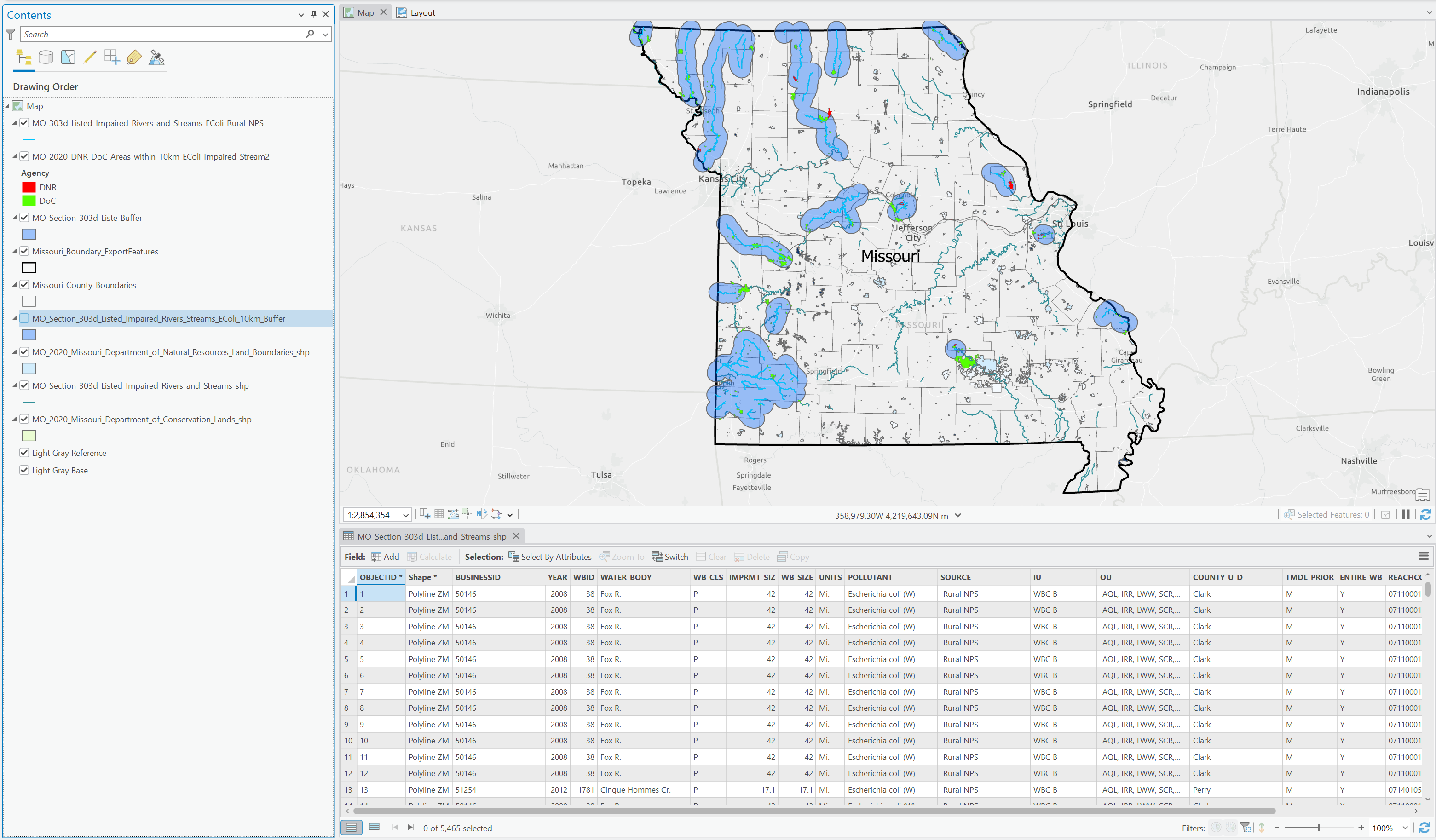
Identified public conservation lands potentially impacted by proximity to E. coli–impaired waterways. Filtered Missouri’s 303(d) list (Rural NPS), generated a 10 km buffer, merged DNR & DoC lands, and intersected to map priority zones.

Precipitation Interpolation and Watershed-Based Rainfall Normalization — Minnesota, August 2007

Landscape Analysis (GEO 669) · ArcGIS Pro · Spatial Analyst · Ordinary Kriging · Zonal Statistics

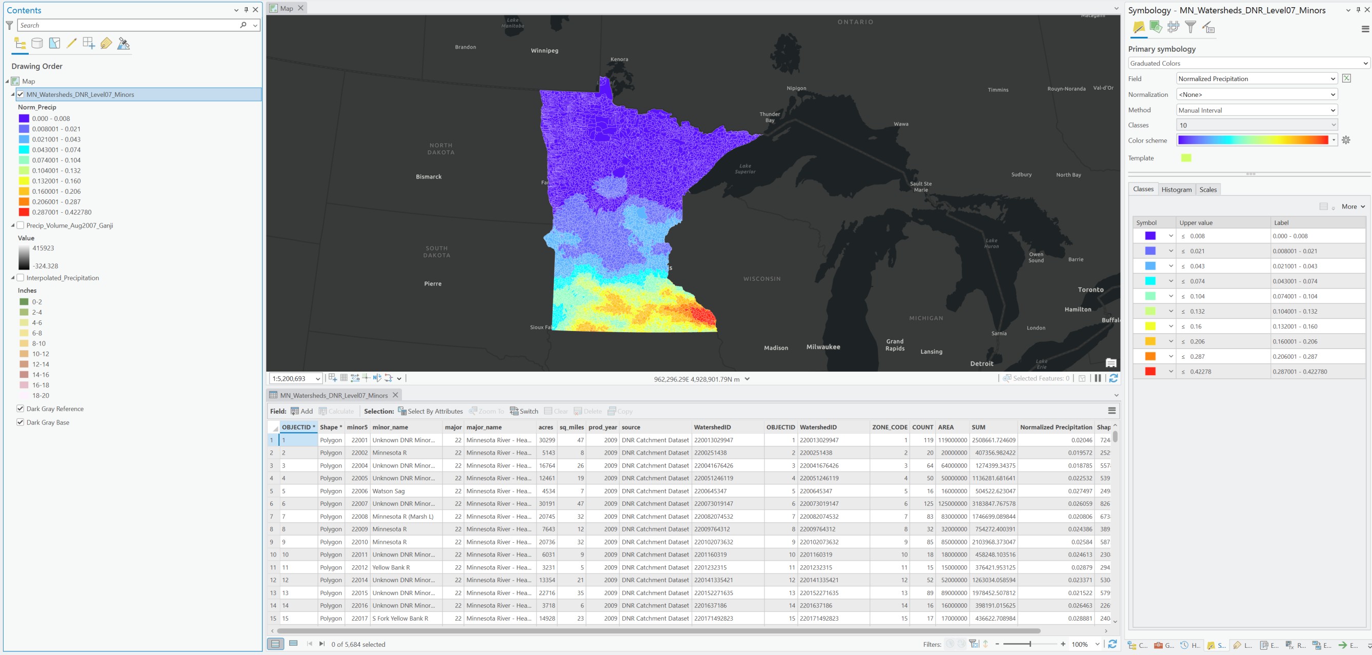
Modeled statewide rainfall distribution from station observations using Ordinary Kriging (Exponential model) in ArcGIS Pro. Converted interpolated precipitation (inches) to rainfall volume (m³) and calculated total and normalized precipitation per Level-07 minor watershed across Minnesota.

Line-of-Sight Viewshed Analysis for Wireless Coverage & Monitoring - Minnesota state,Winona County

Landscape Analysis (GEO 669) · ArcGIS Pro · DEM-based visibility · Observer points & tower height

Overall Objective

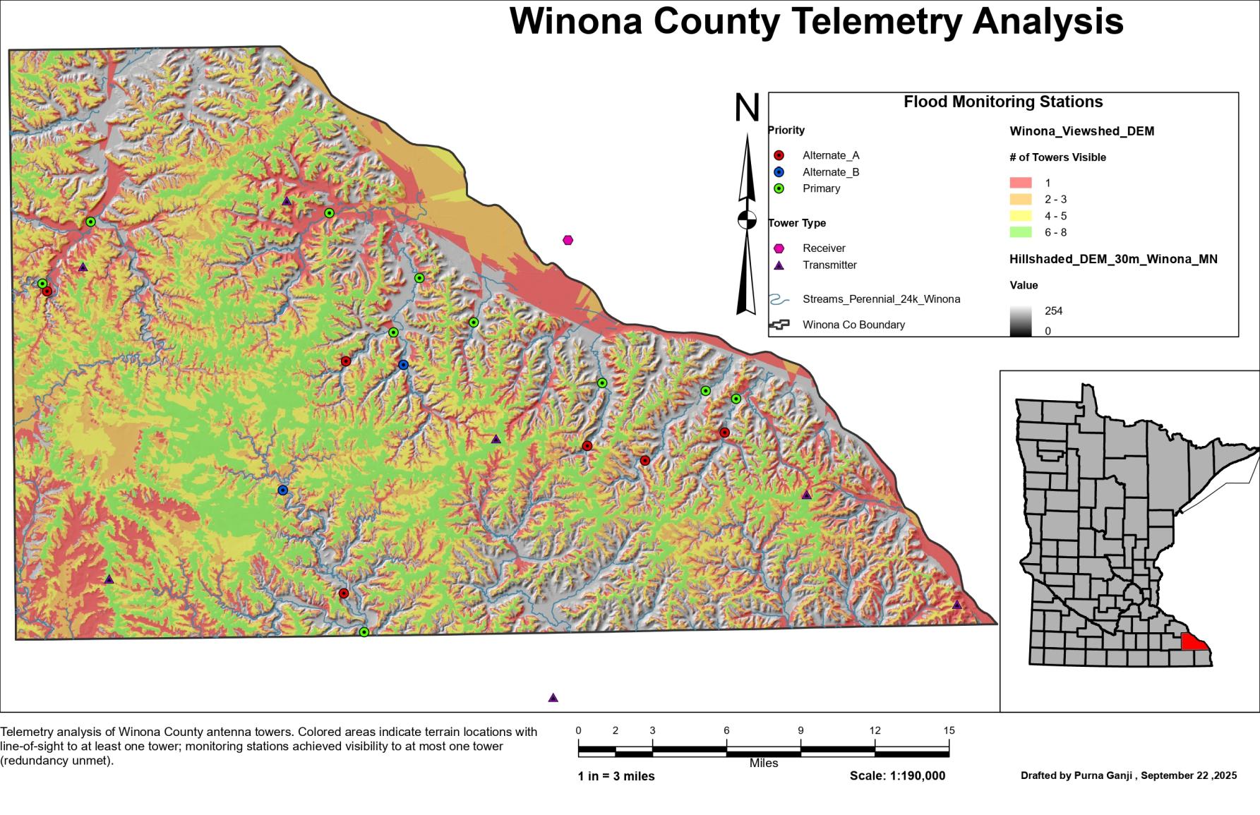
Evaluate whether Winona County flood-monitoring stations can transmit via line-of-sight (LOS) radio to existing 800-MHz antenna towers with redundancy (each station must see ≥ 2 towers). Run a Geodesic Viewshed on a 30-m DEM to quantify visibility, then summarize per-station tower counts to determine viability.

Project Description

1) Study Area Setup

• Created a project geodatabase and added statewide foundational layers.
• Subset to Winona County:
  • Winona County boundary (for map extent and output mask).
  • Clipped 30-m DEM to Winona County; generated hillshade for cartography.
  • National Hydrography Dataset (NHD) Flowline filtered to perennial streams for context.

2) Viewshed Modeling (Physics)

Configured Geodesic Viewshed (accounts for Earth curvature and standard atmospheric refraction) with:

Observer offset (OFFSETA): 305 m (tower antenna height above ground)

Surface/target offset (OFFSETB): 3 m (station antenna height at flood-monitoring site)

Analysis type: Frequency (each raster cell stores the number of towers with LOS to that cell)

Angular limits: Horizontal 0–360°; Vertical +90° to −90° (full dome)

Environments: Snap Raster = DEM; Cell Size = 30 m; Mask = Winona County; Z-factor = 1 (DEM in meters)

3) Per-Station Visibility & Redundancy

• Ran Extract Multi Values to Points to sample the viewshed frequency at each station point.
• Wrote the sampled value to a field TowersSeen (number of towers in LOS from that station).
• Evaluated the redundancy rule: TowersSeen ≥ 2 required for LOS feasibility at each station.

4) Cartography & Communication

• Classified the frequency raster for the map legend using intuitive bins:
  • 1 (single tower)
  • 2–3 (basic redundancy)
  • 4–5 (strong redundancy)
  • 6–8 (excellent redundancy)
• Placed semi-transparent frequency raster over hillshade for terrain context.
• Symbolized stations by priority (meets ≥ 2 towers vs. does not) and towers by type.
• Added perennial streams and a Minnesota inset highlighting Winona County.

Data Sources

• Digital Elevation Model (30 m, statewide): elevation surface used for geodesic viewshed.
• State Boundary (Minnesota): polygon for inset/context.
• County Boundaries (Minnesota): polygons; Winona extracted for mask and extent.
• NHD High Resolution – Flowline: lines; filtered to perennial streams (FCode 46006).
• Antenna Towers (800 MHz): assignment-provided observer points.
• Flood Monitoring Stations: assignment-provided target points.

Coordinate Systems / Projections

• Working / map projection (recommended & used): NAD 1983 / UTM Zone 15N (EPSG: 26915) or NAD 1983 (2011) / UTM Zone 15N (EPSG: 6339).
• Rationale: preserves local distances/areas; keeps DEM units (meters) aligned with offsets (m) and cell size (30 m).
• Raster environment: Cell Size = 30 m, Snap Raster = DEM, Z-factor = 1.
• Output mask: Winona County polygon (tidy outputs and cleaner layout).

Assumptions & QA/QC

• Earth curvature/refraction: geodesic method enabled; standard refractivity assumed.
• Heights: 305 m tower OFFSETA, 3 m station OFFSETB applied consistently.
• DEM suitability: 30-m resolution adequate for county-scale planning; sub-30-m terrain features (buildings/trees) not modeled.
• Layer validation: verified tower and station locations, projected all layers to the working CRS, ensured consistent units.

Results (Findings)

• The frequency viewshed raster returned integer values from 1–6 across Winona County.
• When sampled at station points, TowersSeen was 0 or 1 at all stations (cells with no visibility are NoData and treated as 0 in the table).
• Redundancy test: No stations achieved ≥ 2 towers visible at their current locations – the redundancy requirement was not met.

Conclusion

Given current tower placement and local terrain (bluffs/valleys), LOS telemetry does not provide redundant connectivity for the flood-monitoring stations in Winona County. The county-scale geodesic viewshed on the 30-m DEM indicates stations see at most one tower (or none), failing the ≥ 2-tower redundancy criterion.

Implications / Next Steps

• Network design: Add/relocate towers or repeaters to overcome terrain blocking in valleys.
• Site engineering: Increase station mast heights where feasible; re-site stations onto local ridgelines.
• Alternate backhaul: Evaluate cellular/microwave/satellite where LOS cannot achieve ≥ 2-tower visibility.
• Higher-resolution terrain: Consider LiDAR-derived DEM/DSM with clutter (vegetation/buildings) for micro-siting.
• Sensitivity tests: Re-run viewsheds with varied OFFSETA/OFFSETB, and constrained azimuth/vertical angles.

Garvin Brook Watershed Delineation and Hydrologic Analysis - Minnesota

Surface Hydrology Modeling · ArcGIS Pro · LiDAR DEM · Watershed Delineation

Overall Objective

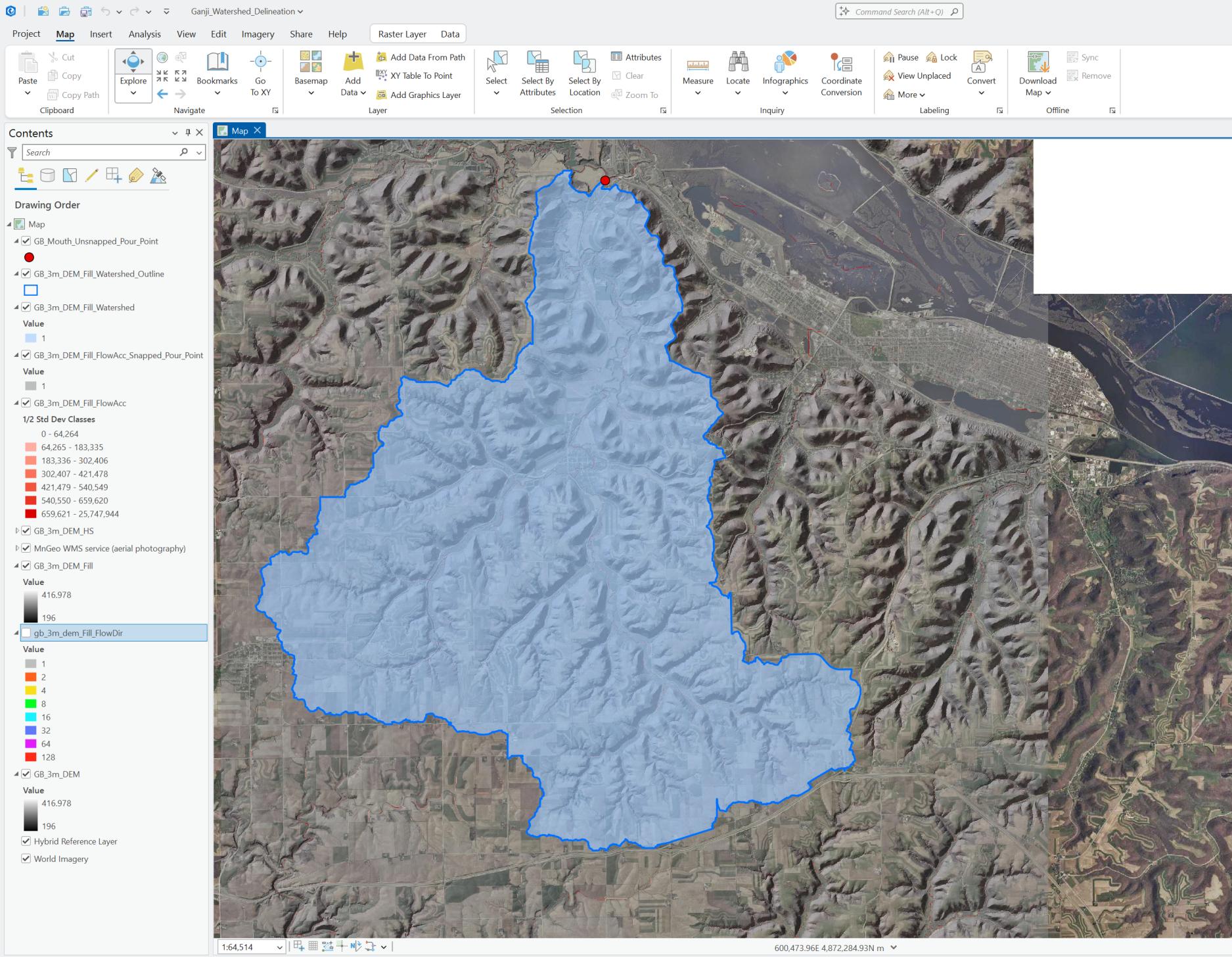
Model surface hydrology using LiDAR-derived elevation data to delineate the Garvin Brook watershed in Minnesota. Process a raw Digital Elevation Model (DEM) into a hydrologically conditioned surface, derive flow direction and flow accumulation grids, and generate an accurate watershed boundary draining to a specific outlet (pour point).

Project Description

1) Data Preparation & Terrain Processing

• Acquired 3-meter LiDAR-derived Digital Elevation Model from Minnesota Geospatial Information Office (MnGeo)
• Created hillshade raster (GB_3m_DEM_HS) for terrain visualization and validation
• Verified coordinate systems and ensured proper raster alignment for analysis

2) Hydrologic Conditioning

Applied Spatial Analyst hydrology tools to create continuous flow surfaces:

• Fill Processing: Removed spurious sinks from DEM to ensure continuous downstream flow
  
• Flow Direction (D8 Algorithm): Established steepest descent path for each cell in the filled DEM
  
• Flow Accumulation: Identified stream channels and contributing areas based on flow direction

3) Watershed Delineation

• Used Snap Pour Point tool to align the watershed outlet to the highest-accumulation channel cell (20 m search radius)
• Executed Watershed tool to delineate the contributing catchment area
• Converted raster watershed to vector polygon boundary for final output

4) Validation & Cartography

• Verified flow paths and watershed boundary against hillshade and aerial imagery
• Applied WMS imagery overlay from MnGeo for base-map context
• Used transparency blending and symbology design to create clear visualization of results

Data Sources

• GB_3m_DEM: 3-meter LiDAR-derived Digital Elevation Model from Minnesota Geospatial Information Office (MnGeo) LiDAR Program
• GB_3m_DEM_HS: Hillshade raster derived from DEM for terrain visualization
• GB_Mouth_Unsnapped_Pour_Point: Initial watershed outlet feature from course dataset
• GB_3m_DEM_Fill_FlowAcc: Pre-generated flow-accumulation raster derived from filled DEM
• MnGeo WMS (2011 Color South MN): Aerial imagery for base-map context from MnGeo Web Map Service

Coordinate Systems / Projections

• Working projection: UTM Zone 15N appropriate for Minnesota regional analysis
• Raster environment: Consistent 3-meter cell size maintained throughout processing
• Alignment: Snap raster settings ensured proper grid alignment for hydrologic tools

Assumptions & QA/QC

• D8 Algorithm: Used single-flow direction model assuming steepest descent path
• Sink Removal: Fill tool applied to eliminate all depressions for continuous flow
• Pour Point Alignment: 20-meter snap distance ensured accurate channel alignment
• Validation: Visual verification of flow paths against terrain and imagery

Results (Findings)

• Successfully generated hydrologically correct DEM (GB_3m_DEM_Fill) with continuous flow paths
• Computed accurate flow-direction grid (gb_3m_dem_Fill_FlowDir) using D8 algorithm
• Aligned pour point to stream channel using Snap Pour Point with 20-meter search radius
• Delineated precise Garvin Brook watershed boundary and converted to polygon format
• Verified watershed accuracy against aerial imagery and terrain features

Conclusion

The hydrologic modeling workflow successfully delineated the Garvin Brook watershed using LiDAR-derived elevation data. The processed DEM and derived flow products provide a reliable foundation for water-resources applications including flood analysis, drainage-area estimation, and stormwater management planning in the Winona County region.

Implications / Next Steps

• Floodplain Mapping: Use watershed boundaries for flood risk assessment and FEMA floodplain delineation
• Stormwater Modeling: Integrate with hydrologic models for runoff and peak flow calculations
• Land Use Planning: Apply watershed analysis for conservation planning and development regulations
• Higher-Resolution Analysis: Consider sub-meter DEM for more detailed channel network mapping
• Multi-direction Flow: Explore D-infinity algorithm for complex terrain situations

Animated Spatiotemporal Visualization of September Air Temperatures in China (1854–2014)

Climate Data Analysis · ArcGIS Pro · Kriging Interpolation · Temporal Animation

Overall Objective

Model, visualize, and animate the long-term spatial and temporal patterns of September air temperature across China from 1854 to 2014 using kriging interpolation and consistent symbology parameters, enabling clear communication of historical climate trends through geospatial animation.

Project Description

1) Data Processing & Preparation

• Collected point temperature data spanning 160 years (1854-2014) for September months
• Processed and organized temporal data into decadal intervals in ArcGIS Pro
• Applied uniform coordinate system (WGS 1984 Web Mercator Auxiliary Sphere) for spatial consistency

2) Spatial Interpolation & Surface Generation

Applied geostatistical analysis to create continuous temperature surfaces:

Ordinary Kriging:

Used Spatial Analyst Toolbox for optimal interpolation of point temperature data

Raster Generation:

Created 17 individual raster surfaces representing each time period

Quality Control:

Validated interpolation results against original point data

3) Cartographic Standardization

• Applied consistent symbology range (273 K – 308 K) across all 17 raster maps
• Overlaid China and neighboring country boundaries for geographic context
• Exported all maps as high-resolution PNG images at 300 DPI

4) Animation Production

• Compiled 17 raster maps into sequential animation using Python-based automation
• Configured one-second display per frame with smooth fade transitions
• Produced final animated visualization showing spatial and temporal temperature evolution

Data Sources

• Historical Temperature Records: Point temperature data for China (1854-2014)
• Administrative Boundaries: China and neighboring country polygons for map context
• Base Cartography: Reference layers for geographic orientation

Coordinate Systems / Projections

• Primary Projection: WGS 1984 Web Mercator Auxiliary Sphere
• Rationale: Ensured spatial consistency across all temporal outputs
• Standardization: Uniform coordinate reference for accurate temporal comparison

Assumptions & QA/QC

• Interpolation Method: Ordinary Kriging provided optimal surface estimation
• Temporal Resolution: Decadal intervals adequately captured climate trends
• Data Consistency: Measurement methods consistent across 160-year period
• Visual Validation: Manual verification of interpolation results against source data

Results (Findings)

• Successfully generated 17 temporally sequential temperature surfaces
• Revealed persistent north–south temperature gradient across all time periods
• Detected northward shift of warmer zones over the decades
• Identified progressive warming trend consistent with observed climate change patterns
• Produced compelling animated visualization bridging scientific analysis and visual storytelling

Conclusion

The spatiotemporal animation successfully visualized 160 years of September temperature patterns across China, clearly demonstrating both spatial gradients and temporal warming trends. The methodology combining kriging interpolation with standardized cartography and animation techniques proved effective for communicating complex climate data through intuitive visual storytelling.

Implications / Next Steps

• Climate Communication: Enhanced tools for communicating climate change impacts to diverse audiences
• Educational Applications: Valuable resource for climate science education and public awareness
• Methodological Expansion: Apply similar techniques to other climate variables and geographic regions
• Higher Temporal Resolution: Explore monthly or seasonal patterns beyond September data
• Interactive Development: Create web-based interactive versions for broader accessibility